Performans ölçümü, makine öğrenmesi süreçlerinde geliştirilen modellerin gerçek dünya verileri üzerinde ne kadar etkili olduğunu değerlendirmemize olanak tanıyarak makine öğrenmesi süreçlerinde hayati bir rol oynar. Performans ölçümü, bir modelin doğruluğunu, genelleme yeteneğini ve veri uyumunu belirleyerek, algoritmaların ve yapılandırmaların ne kadar etkili olduğunu anlamamıza yardımcı olur. Performans ölçümü aynı zamanda karar verme süreçlerinde güvenilirliği artırır, çünkü modellerin gerçek dünya koşullarında ne kadar iyi performans gösterdiğini belirler. Dolayısıyla performans ölçümü, makine öğrenmesi projelerinde başarının anahtarını oluşturur, çünkü geliştirilen modellerin gerçek dünya problemlerine ne kadar uygun olduğunu objektif bir şekilde değerlendirme imkânı sağlar. Bu nedenle, yapay zekâ projelerinde performans ölçümünün titizlikle yapılması ve doğru metriklerin seçilmesi büyük önem taşır.
Makine öğrenmesinde kullanılan metrikler, modellerin etkinliğini ve güvenilirliğini değerlendirmek için temel bir unsurdur ve her makine öğrenmesi sürecinde bulunurlar. Doğru performans metriklerini belirlemek, projenin başarısını ölçmek ve algoritmaları geliştirmek için kritiktir. Bu yazıda hem regresyon hem de sınıflandırma problemleri için önde gelen performans metrikleri incelenmiş ve model performansı hakkında hangi bilgileri sağladıkları ele alınmıştır. Böylece kullanım durumuna göre en uygun metrikleri seçebilirsiniz.
Bazı önde gelen performans metriklerine örnek vermek gerekirse bunlar: Doğruluk (Accuracy), Kesinlik (Precision), Duyarlılık (Recall/Sensitivity), F1-Skoru (F1-Score), ROC Eğrisi ve AUC (Receiver Operating Characteristic Curve and Area Under the Curve), RMSE (Root Mean Square Error), MAE (Mean Absolute Error), R-Kare (R-Squared).
Makine öğrenmesinde en sık kullanılan bazı metrikler:
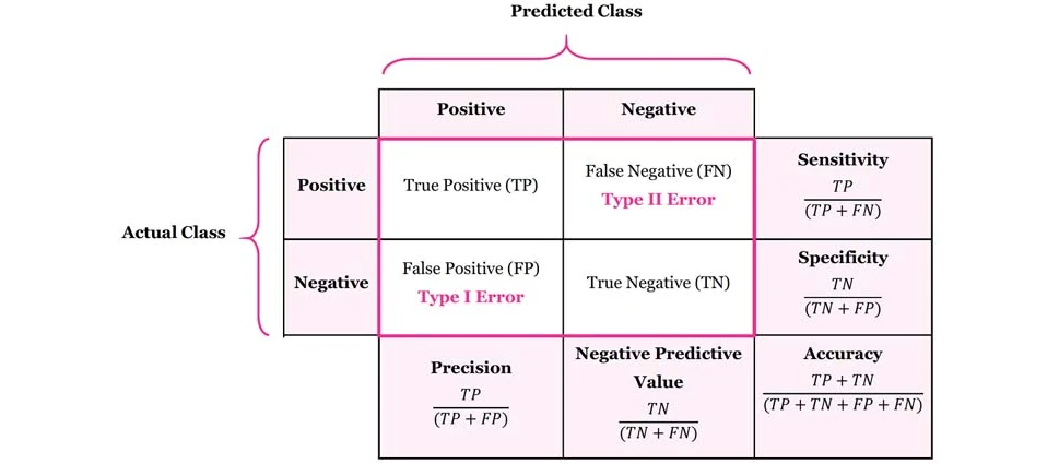
- Doğruluk (Accuracy), bir sınıflandırma modelinin toplam tahminler içinde doğru tahminlerin oranını temsil eder. Doğruluk değeri modelin ne kadar iyi çalıştığını genel bir bakış açısıyla değerlendirmeye yardımcı olur. Ancak doğruluk tek başına modelin performansını tam olarak göstermeyebilir çünkü sınıflandırma dengesizliği durumlarında yanıltıcı olabilir. Diğer bir deyişle, modelin sınıflandırma yaparken yanlış tahmin ettiği pozitif (1) ve negatif (0) örneklerin sayılarına dikkat etmek önemlidir.
True Positive (TP), gerçekte pozitif olan örnekleri doğru bir şekilde pozitif olarak tahmin etme durumunu ifade eder. True Negative (TN), gerçekte negatif olan örnekleri doğru bir şekilde negatif olarak tahmin etme durumunu ifade eder. False Positive (FP), gerçekte negatif olan örnekleri yanlış bir şekilde pozitif olarak tahmin etme durumunu ifade eder. False Negative (FN), gerçekte pozitif olan örnekleri yanlış bir şekilde negatif olarak tahmin etme durumunu ifade eder.
Doğruluk metriği, bu dört durumu dikkate alarak, modelin doğru tahmin etme yeteneğini değerlendirir. Ancak, dengesiz veri setleri veya maliyet odaklı problemler gibi durumlarda doğruluk tek başına yetersiz olabilir. Bu nedenle, modelin performansını daha ayrıntılı bir şekilde değerlendirmek için diğer metriklerle birlikte kullanılması daha sağlıklı olacaktır.
- Kesinlik (Precision), bir sınıflandırma modelinin pozitif olarak tahmin ettiği örneklerin gerçekte ne kadarının pozitif olduğunu ölçer. Kesinlik, yanlış pozitif tahminlerin sayısını azaltmaya odaklanır ve bu nedenle modelin gerçek pozitifleri doğru bir şekilde tespit etme yeteneğini değerlendirir. Kesinlik, özellikle yanlış pozitif tahminlerin maliyeti yüksek olduğu durumlarda önemlidir, örneğin, tıbbi teşhisler veya dolandırıcılık tespiti gibi alanlarda. Dolayısıyla kesinlik metriği, modelin güvenilirliğini değerlendirmek ve yanlış pozitiflerin sayısını en aza indirmek için kullanılmalıdır.
- Duyarlılık (Recall/Sensitivity), bir sınıflandırma modelinin gerçek pozitiflerin ne kadarını doğru bir şekilde tespit ettiğini ölçer. Duyarlılık, yanlış negatif tahminlerin sayısını azaltmaya odaklanır ve modelin gerçek pozitifleri kaçırmama yeteneğini değerlendirir. Özellikle, yanlış negatif tahminlerin ciddi sonuçlara yol açtığı durumlarda, örneğin, tıbbi teşhisler veya güvenlik uygulamaları gibi alanlarda, duyarlılık metriği önemlidir. Bu nedenle, modelin duyarlılığını değerlendirmek ve gerçek pozitifleri kaçırma riskini azaltmak için duyarlılık metriği kullanılmalıdır.
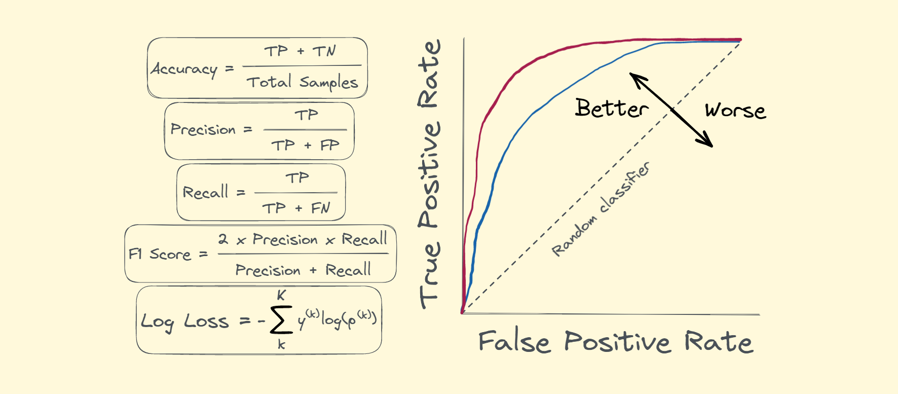
- F1-Skoru (F1-Score), bir sınıflandırma modelinin kesinlik (precision) ve duyarlılık (recall) performanslarının birleşik bir ölçüsünü sağlar. F1-Skoru, hem yanlış pozitiflerin hem de yanlış negatiflerin etkisini dengeler ve bu nedenle modelin genel performansını daha iyi bir şekilde değerlendirir. F1-Skoru, modelin hem doğruluğunu hem de gerçek pozitifleri kaçırma riskini dikkate alır. Özellikle, dengesiz sınıflandırma problemleri veya farklı maliyetlerin olduğu durumlarda, F1-Skoru kullanılmalıdır.
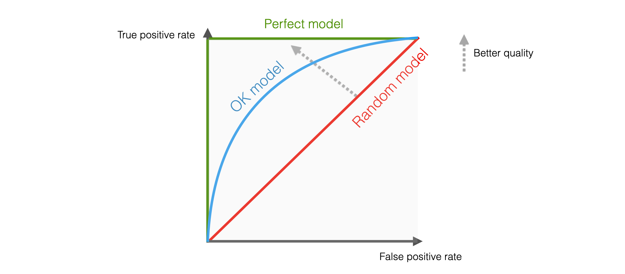
- ROC Eğrisi ve AUC (Receiver Operating Characteristic Curve and Area Under the Curve), bir sınıflandırma modelinin performansını değerlendirmek için yaygın olarak kullanılan görsel ve nicel bir metriktir. ROC Eğrisi, sınıflandırma modelinin farklı kesme noktalarında duyarlılık (recall) ile yanlış pozitif oranı (false positive rate) arasındaki ilişkiyi gösteren bir grafiktir. ROC eğrisi, modelin farklı duyarlılık ve özgüllük (specificity) düzeylerindeki performansını görsel olarak gösterir. Kesme noktalarının seçimi, modelin hassasiyetini veya özgüllüğünü ayarlamak için kullanılabilir ve karar verme sürecinde esneklik sağlar. AUC (Area Under the Curve), ROC eğrisinin altındaki alanı ifade eder. AUC, sınıflandırma modelinin tüm duyarlılık ve özgüllük düzeylerindeki performansını tek bir numaraya indirger. AUC değeri genellikle 0 ile 1 arasında değişir; 1'e yaklaşan bir AUC değeri, modelin mükemmel bir performansa sahip olduğunu, 0.5'e yaklaşan bir değer ise rastgele tahmin etmekle eşdeğer olduğunu gösterir. Bu nedenle, AUC değeri, sınıflandırma modelinin genel performansını ölçmek için kullanılan bir ölçüdür. ROC Eğrisi ve AUC, özellikle dengesiz sınıflandırma problemlerinde ve farklı kesme noktalarının performans üzerinde farklı etkilere sahip olduğu durumlarda kullanışlıdır. Bu metrikler, modelin duyarlılık ve özgüllük düzeylerindeki performansını anlamak ve optimize etmek için önemli bir yol sağlar.
- RMSE (Root Mean Square Error), regresyon modellerinin tahmin performansını değerlendirmek için kullanılan bir metriktir. RMSE, modelin gerçek değerlerle tahmin edilen değerler arasındaki farkları ölçer ve bu farkların standart sapmasını hesaplar. Özellikle, tahmin hatalarının önemli olduğu durumlarda, örneğin, finansal tahminlerde veya doğal fenomenlerin modellenmesinde, RMSE değerlendirme için tercih edilir.
- MAE (Mean Absolute Error), regresyon modellerinin tahmin performansını değerlendirmek için kullanılan bir metriktir. MAE, modelin gerçek değerlerle tahmin edilen değerler arasındaki farkların mutlak değerlerinin ortalamasını hesaplar. Özellikle, aykırı değerlerin olduğu durumlarda RMSE'ye göre daha dirençli olduğu için, MAE tercih edilebilir.
- R-Kare (R-Squared), regresyon modellerinin bağımsız değişkenler tarafından açıklanan bağımlı değişkenin varyansının oranını ifade eden bir metriktir. R-Kare, bir modelin ne kadar iyi uyum sağladığını gösterir; yüksek bir R-Kare değeri, modelin veriye daha iyi uyum sağladığını, düşük bir R-Kare değeri ise modelin veriye uyum sağlama yeteneğinin daha zayıf olduğunu gösterir. Bu nedenle, R-Kare, regresyon modellerinin performansını değerlendirmek ve karşılaştırmak için kullanılır.
Sonuç olarak, performans ölçümü makine öğrenmesi projelerindeki başarıyı değerlendirmek için kritik bir rol oynar. Amaca uygun seçilen metrikler, geliştirilen modellerin gerçek dünya verileri üzerinde ne kadar etkili olduğunu belirlememize yardımcı olur. Doğru performans metriklerinin seçilmesi, modelin doğruluğunu, genelleme yeteneğini ve veri uyumunu anlamamıza olanak tanır. Önde gelen performans metrikleri arasında doğruluk, kesinlik, duyarlılık, F1-Skoru, ROC Eğrisi ve AUC, RMSE, MAE ve R-Kare bulunmaktadır. Bu metrikler, hem sınıflandırma hem de regresyon problemleri için önemlidir ve her biri farklı bilgiler sağlar. Doğru metrikleri seçmek, projenizin başarısını ölçmek ve algoritmalarınızı geliştirmek için hayati önem taşır. Dolayısıyla makine öğrenmesi projelerinde performans ölçümünün titizlikle yapılması ve uygun metriklerin seçilmesi gerekmektedir.


.png)


.png)
.png)


 Kelime Gömmeleri (Word Embeddings)


 SMEMA Nedir?
.png)
.png)